Python numpy histogram2d用法及代码示例

本文简要介绍 python 语言中 numpy.histogram2d 的用法。

用法:

numpy.histogram2d(x, y, bins=10, range=None, normed=None, weights=None, density=None)

计算两个数据样本的二维直方图。

参数：

x： 数组, 形状 (N,)

包含要进行直方图分析的点的 x 坐标的数组。

y： 数组, 形状 (N,)

包含要直方图的点的 y 坐标的数组。

bins： int or 数组 or [int, int] or [array, array], 可选

箱规格：

• 如果是 int，则为二维的 bin 数量 (nx=ny=bins)。

• 如果 数组，则两个维度的 bin 边 (x_edges=y_edges=bins)。

• 如果 [int, int]，每个维度的 bin 数(nx, ny = bins)。

• 如果 [array, array]，则每个维度中的 bin 边 (x_edges, y_edges = bins)。

• [int, array] 或 [array, int] 的组合，其中 int 是 bin 的数量，array 是 bin 的边。

range： 数组，形状(2,2)，可选

沿每个维度的 bin 的最左侧和最右侧边(如果未在箱子参数)：[[xmin, xmax], [ymin, ymax]].此范围之外的所有值都将被视为异常值，并且不计入直方图中。

density： 布尔型，可选

如果默认为 False，则返回每个 bin 中的样本数。如果为真，则返回概率密度函数在箱子，bin_count / sample_count / bin_area.

normed： 布尔型，可选

行为相同的密度参数的别名。为了避免与破坏的规范论证混淆numpy.histogram,密度应该是首选。

weights： 数组，形状(N，)，可选

一组值w_i称量每个样品(x_i, y_i).如果权重归一化为 1规范的是真的。如果规范的为 False，返回的直方图的值等于属于每个 bin 的样本的权重之和。

返回：

H： ndarray，形状(nx，ny)

样本 x 和 y 的二维直方图。 x 中的值沿第一维进行直方图，y 中的值沿第二维进行直方图。

xedges： ndarray，形状(nx+1，)

bin 沿第一个维度边。

yedges： ndarray，形状(ny+1，)

箱沿第二个维度边。

注意：

什么时候规范的为 True，则返回的直方图是样本密度，定义为使得产品的 bin 上的总和bin_value * bin_area是 1。

请注意，直方图不遵循笛卡尔约定，其中x值在横坐标和y纵坐标轴上的值。相当，x沿数组的第一个维度(垂直)进行直方图，并且y沿数组的第二维(水平)。这确保了与numpy.histogramdd.

例子：

>>> from matplotlib.image import NonUniformImage
>>> import matplotlib.pyplot as plt

构建具有可变 bin 宽度的二维直方图。首先定义 bin 边：

>>> xedges = [0, 1, 3, 5]
>>> yedges = [0, 2, 3, 4, 6]

接下来我们创建一个带有随机 bin 内容的直方图 H：

>>> x = np.random.normal(2, 1, 100)
>>> y = np.random.normal(1, 1, 100)
>>> H, xedges, yedges = np.histogram2d(x, y, bins=(xedges, yedges))
>>> # Histogram does not follow Cartesian convention (see Notes),
>>> # therefore transpose H for visualization purposes.
>>> H = H.T

imshow 只能显示方形箱：

>>> fig = plt.figure(figsize=(7, 3))
>>> ax = fig.add_subplot(131, title='imshow: square bins')
>>> plt.imshow(H, interpolation='nearest', origin='lower',
...         extent=[xedges[0], xedges[-1], yedges[0], yedges[-1]])
<matplotlib.image.AxesImage object at 0x...>

pcolormesh 可以显示实际边：

>>> ax = fig.add_subplot(132, title='pcolormesh: actual edges',
...         aspect='equal')
>>> X, Y = np.meshgrid(xedges, yedges)
>>> ax.pcolormesh(X, Y, H)
<matplotlib.collections.QuadMesh object at 0x...>

NonUniformImage 可用于显示带有插值的实际 bin 边：

>>> ax = fig.add_subplot(133, title='NonUniformImage: interpolated',
...         aspect='equal', xlim=xedges[[0, -1]], ylim=yedges[[0, -1]])
>>> im = NonUniformImage(ax, interpolation='bilinear')
>>> xcenters = (xedges[:-1] + xedges[1:]) / 2
>>> ycenters = (yedges[:-1] + yedges[1:]) / 2
>>> im.set_data(xcenters, ycenters, H)
>>> ax.images.append(im)
>>> plt.show()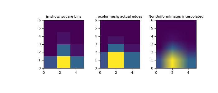

也可以在不指定 bin 边的情况下构造二维直方图：

>>> # Generate non-symmetric test data
>>> n = 10000
>>> x = np.linspace(1, 100, n)
>>> y = 2*np.log(x) + np.random.rand(n) - 0.5
>>> # Compute 2d histogram. Note the order of x/y and xedges/yedges
>>> H, yedges, xedges = np.histogram2d(y, x, bins=20)

现在我们可以使用 pcolormesh 和 hexbin 绘制直方图以进行比较。

>>> # Plot histogram using pcolormesh
>>> fig, (ax1, ax2) = plt.subplots(ncols=2, sharey=True)
>>> ax1.pcolormesh(xedges, yedges, H, cmap='rainbow')
>>> ax1.plot(x, 2*np.log(x), 'k-')
>>> ax1.set_xlim(x.min(), x.max())
>>> ax1.set_ylim(y.min(), y.max())
>>> ax1.set_xlabel('x')
>>> ax1.set_ylabel('y')
>>> ax1.set_title('histogram2d')
>>> ax1.grid()

>>> # Create hexbin plot for comparison
>>> ax2.hexbin(x, y, gridsize=20, cmap='rainbow')
>>> ax2.plot(x, 2*np.log(x), 'k-')
>>> ax2.set_title('hexbin')
>>> ax2.set_xlim(x.min(), x.max())
>>> ax2.set_xlabel('x')
>>> ax2.grid()

>>> plt.show()