Augment 接受模型對象和數據集,並添加有關數據集中每個觀察值的信息。最常見的是,這包括 .fitted 列中的預測值、.resid 列中的殘差以及 .se.fit 列中擬合值的標準誤差。新列始終以 . 前綴開頭,以避免覆蓋原始數據集中的列。
用戶可以通過 data 參數或 newdata 參數傳遞數據以進行增強。如果用戶將數據傳遞給 data 參數,則它必須正是用於擬合模型對象的數據。將數據集傳遞給 newdata 以擴充模型擬合期間未使用的數據。這仍然要求至少存在用於擬合模型的所有預測變量列。如果用於擬合模型的原始結果變量未包含在 newdata 中,則輸出中不會包含 .resid 列。
根據是否給出 data 或 newdata,增強的行為通常會有所不同。這是因為通常存在與訓練觀察(例如影響或相關)測量相關的信息,而這些信息對於新觀察沒有有意義的定義。
為了方便起見,許多增強方法提供默認的 data 參數,以便 augment(fit) 將返回增強的訓練數據。在這些情況下,augment 嘗試根據模型對象重建原始數據,並取得了不同程度的成功。
增強數據集始終以 tibble::tibble 形式返回,其行數與傳遞的數據集相同。這意味著傳遞的數據必須可強製轉換為 tibble。如果預測變量將模型作為協變量矩陣的一部分輸入,例如當模型公式使用 splines::ns() 、 stats::poly() 或 survival::Surv() 時,它會表示為矩陣列。
我們正在定義適合各種 na.action 參數的模型的行為,但目前不保證數據丟失時的行為。
參數
- x
-
從
poLCA::poLCA()返回的poLCA對象。 - data
-
base::data.frame 或
tibble::tibble()包含用於生成對象x的原始數據。默認為stats::model.frame(x),以便augment(my_fit)返回增強的原始數據。不要將新數據傳遞給data參數。增強將報告傳遞給data參數的數據的影響和烹飪距離等信息。這些度量僅針對原始訓練數據定義。 - ...
-
附加參數。不曾用過。僅需要匹配通用簽名。注意:拚寫錯誤的參數將被吸收到
...中,並被忽略。如果拚寫錯誤的參數有默認值,則將使用默認值。例如,如果您傳遞conf.lvel = 0.9,所有計算將使用conf.level = 0.95進行。這裏有兩個異常:
細節
如果給出 data 參數,則這些列將包含在輸出中(僅可以進行預測的行)。否則,將使用 poLCA 對象的 y 元素(其中包含用於擬合模型的清單變量)以及 x 中的任何協變量(如果存在)。
請注意,雖然所有類(不僅僅是預測模態類)的概率都可以在 posterior 元素中找到,但這些不包含在增強輸出中。
也可以看看
其他 poLCA 整理器:glance.poLCA() 、tidy.poLCA()
例子
# load libraries for models and data
library(poLCA)
#> Loading required package: scatterplot3d
library(dplyr)
# generate data
data(values)
f <- cbind(A, B, C, D) ~ 1
# fit model
M1 <- poLCA(f, values, nclass = 2, verbose = FALSE)
M1
#> Conditional item response (column) probabilities,
#> by outcome variable, for each class (row)
#>
#> $A
#> Pr(1) Pr(2)
#> class 1: 0.2864 0.7136
#> class 2: 0.0068 0.9932
#>
#> $B
#> Pr(1) Pr(2)
#> class 1: 0.6704 0.3296
#> class 2: 0.0602 0.9398
#>
#> $C
#> Pr(1) Pr(2)
#> class 1: 0.6460 0.3540
#> class 2: 0.0735 0.9265
#>
#> $D
#> Pr(1) Pr(2)
#> class 1: 0.8676 0.1324
#> class 2: 0.2309 0.7691
#>
#> Estimated class population shares
#> 0.7208 0.2792
#>
#> Predicted class memberships (by modal posterior prob.)
#> 0.6713 0.3287
#>
#> =========================================================
#> Fit for 2 latent classes:
#> =========================================================
#> number of observations: 216
#> number of estimated parameters: 9
#> residual degrees of freedom: 6
#> maximum log-likelihood: -504.4677
#>
#> AIC(2): 1026.935
#> BIC(2): 1057.313
#> G^2(2): 2.719922 (Likelihood ratio/deviance statistic)
#> X^2(2): 2.719764 (Chi-square goodness of fit)
#>
# summarize model fit with tidiers + visualization
tidy(M1)
#> # A tibble: 16 × 5
#> variable class outcome estimate std.error
#> <chr> <int> <dbl> <dbl> <dbl>
#> 1 A 1 1 0.286 0.0393
#> 2 A 2 1 0.00681 0.0254
#> 3 A 1 2 0.714 0.0393
#> 4 A 2 2 0.993 0.0254
#> 5 B 1 1 0.670 0.0489
#> 6 B 2 1 0.0602 0.0649
#> 7 B 1 2 0.330 0.0489
#> 8 B 2 2 0.940 0.0649
#> 9 C 1 1 0.646 0.0482
#> 10 C 2 1 0.0735 0.0642
#> 11 C 1 2 0.354 0.0482
#> 12 C 2 2 0.927 0.0642
#> 13 D 1 1 0.868 0.0379
#> 14 D 2 1 0.231 0.0929
#> 15 D 1 2 0.132 0.0379
#> 16 D 2 2 0.769 0.0929
augment(M1)
#> # A tibble: 216 × 7
#> A B C D X.Intercept. .class .probability
#> <dbl> <dbl> <dbl> <dbl> <dbl> <int> <dbl>
#> 1 2 2 2 2 1 2 0.959
#> 2 2 2 2 2 1 2 0.959
#> 3 2 2 2 2 1 2 0.959
#> 4 2 2 2 2 1 2 0.959
#> 5 2 2 2 2 1 2 0.959
#> 6 2 2 2 2 1 2 0.959
#> 7 2 2 2 2 1 2 0.959
#> 8 2 2 2 2 1 2 0.959
#> 9 2 2 2 2 1 2 0.959
#> 10 2 2 2 2 1 2 0.959
#> # ℹ 206 more rows
glance(M1)
#> # A tibble: 1 × 8
#> logLik AIC BIC g.squared chi.squared df df.residual nobs
#> <dbl> <dbl> <dbl> <dbl> <dbl> <dbl> <dbl> <int>
#> 1 -504. 1027. 1057. 2.72 2.72 9 6 216
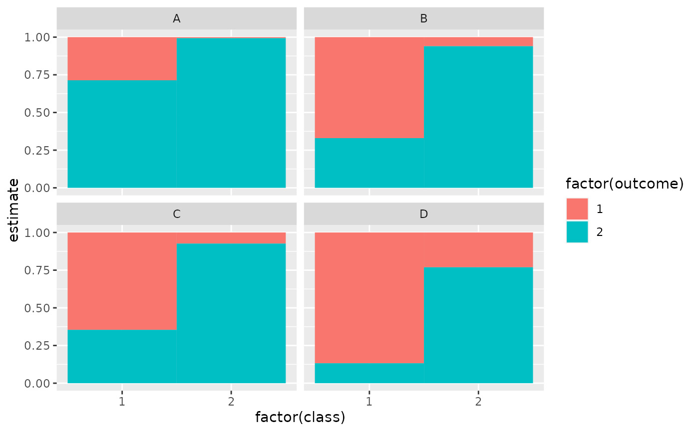
library(ggplot2)
ggplot(tidy(M1), aes(factor(class), estimate, fill = factor(outcome))) +
geom_bar(stat = "identity", width = 1) +
facet_wrap(~variable)
 # three-class model with a single covariate.
data(election)
f2a <- cbind(
MORALG, CARESG, KNOWG, LEADG, DISHONG, INTELG,
MORALB, CARESB, KNOWB, LEADB, DISHONB, INTELB
) ~ PARTY
nes2a <- poLCA(f2a, election, nclass = 3, nrep = 5, verbose = FALSE)
td <- tidy(nes2a)
td
#> # A tibble: 144 × 5
#> variable class outcome estimate std.error
#> <chr> <int> <fct> <dbl> <dbl>
#> 1 MORALG 1 1 Extremely well 0.108 0.0175
#> 2 MORALG 2 1 Extremely well 0.137 0.0182
#> 3 MORALG 3 1 Extremely well 0.622 0.0309
#> 4 MORALG 1 2 Quite well 0.383 0.0274
#> 5 MORALG 2 2 Quite well 0.668 0.0247
#> 6 MORALG 3 2 Quite well 0.335 0.0293
#> 7 MORALG 1 3 Not too well 0.304 0.0253
#> 8 MORALG 2 3 Not too well 0.180 0.0208
#> 9 MORALG 3 3 Not too well 0.0172 0.00841
#> 10 MORALG 1 4 Not well at all 0.205 0.0243
#> # ℹ 134 more rows
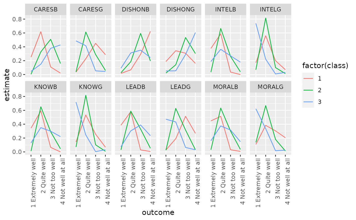
ggplot(td, aes(outcome, estimate, color = factor(class), group = class)) +
geom_line() +
facet_wrap(~variable, nrow = 2) +
theme(axis.text.x = element_text(angle = 90, hjust = 1))
# three-class model with a single covariate.
data(election)
f2a <- cbind(
MORALG, CARESG, KNOWG, LEADG, DISHONG, INTELG,
MORALB, CARESB, KNOWB, LEADB, DISHONB, INTELB
) ~ PARTY
nes2a <- poLCA(f2a, election, nclass = 3, nrep = 5, verbose = FALSE)
td <- tidy(nes2a)
td
#> # A tibble: 144 × 5
#> variable class outcome estimate std.error
#> <chr> <int> <fct> <dbl> <dbl>
#> 1 MORALG 1 1 Extremely well 0.108 0.0175
#> 2 MORALG 2 1 Extremely well 0.137 0.0182
#> 3 MORALG 3 1 Extremely well 0.622 0.0309
#> 4 MORALG 1 2 Quite well 0.383 0.0274
#> 5 MORALG 2 2 Quite well 0.668 0.0247
#> 6 MORALG 3 2 Quite well 0.335 0.0293
#> 7 MORALG 1 3 Not too well 0.304 0.0253
#> 8 MORALG 2 3 Not too well 0.180 0.0208
#> 9 MORALG 3 3 Not too well 0.0172 0.00841
#> 10 MORALG 1 4 Not well at all 0.205 0.0243
#> # ℹ 134 more rows
ggplot(td, aes(outcome, estimate, color = factor(class), group = class)) +
geom_line() +
facet_wrap(~variable, nrow = 2) +
theme(axis.text.x = element_text(angle = 90, hjust = 1))
 au <- augment(nes2a)
au
#> # A tibble: 1,300 × 16
#> MORALG CARESG KNOWG LEADG DISHONG INTELG MORALB CARESB KNOWB LEADB
#> <fct> <fct> <fct> <fct> <fct> <fct> <fct> <fct> <fct> <fct>
#> 1 3 Not too … 1 Ext… 2 Qu… 2 Qu… 3 Not … 2 Qui… 1 Ext… 1 Ext… 2 Qu… 2 Qu…
#> 2 1 Extremel… 2 Qui… 2 Qu… 1 Ex… 3 Not … 2 Qui… 2 Qui… 2 Qui… 2 Qu… 3 No…
#> 3 2 Quite we… 2 Qui… 2 Qu… 2 Qu… 2 Quit… 2 Qui… 2 Qui… 3 Not… 2 Qu… 2 Qu…
#> 4 2 Quite we… 4 Not… 2 Qu… 3 No… 2 Quit… 2 Qui… 1 Ext… 1 Ext… 2 Qu… 2 Qu…
#> 5 2 Quite we… 2 Qui… 2 Qu… 2 Qu… 3 Not … 2 Qui… 3 Not… 4 Not… 4 No… 4 No…
#> 6 2 Quite we… 2 Qui… 2 Qu… 3 No… 4 Not … 2 Qui… 2 Qui… 3 Not… 2 Qu… 2 Qu…
#> 7 1 Extremel… 1 Ext… 1 Ex… 1 Ex… 4 Not … 1 Ext… 2 Qui… 4 Not… 2 Qu… 3 No…
#> 8 2 Quite we… 2 Qui… 2 Qu… 2 Qu… 3 Not … 2 Qui… 3 Not… 2 Qui… 2 Qu… 2 Qu…
#> 9 2 Quite we… 2 Qui… 2 Qu… 2 Qu… 3 Not … 2 Qui… 2 Qui… 2 Qui… 2 Qu… 3 No…
#> 10 2 Quite we… 3 Not… 2 Qu… 2 Qu… 3 Not … 2 Qui… 2 Qui… 4 Not… 2 Qu… 4 No…
#> # ℹ 1,290 more rows
#> # ℹ 6 more variables: DISHONB <fct>, INTELB <fct>, X.Intercept. <dbl>,
#> # PARTY <dbl>, .class <int>, .probability <dbl>
count(au, .class)
#> # A tibble: 3 × 2
#> .class n
#> <int> <int>
#> 1 1 444
#> 2 2 496
#> 3 3 360
# if the original data is provided, it leads to NAs in new columns
# for rows that weren't predicted
au2 <- augment(nes2a, data = election)
au2
#> # A tibble: 1,785 × 20
#> MORALG CARESG KNOWG LEADG DISHONG INTELG MORALB CARESB KNOWB LEADB
#> <fct> <fct> <fct> <fct> <fct> <fct> <fct> <fct> <fct> <fct>
#> 1 3 Not too … 1 Ext… 2 Qu… 2 Qu… 3 Not … 2 Qui… 1 Ext… 1 Ext… 2 Qu… 2 Qu…
#> 2 4 Not well… 3 Not… 4 No… 3 No… 2 Quit… 2 Qui… NA NA 2 Qu… 3 No…
#> 3 1 Extremel… 2 Qui… 2 Qu… 1 Ex… 3 Not … 2 Qui… 2 Qui… 2 Qui… 2 Qu… 3 No…
#> 4 2 Quite we… 2 Qui… 2 Qu… 2 Qu… 2 Quit… 2 Qui… 2 Qui… 3 Not… 2 Qu… 2 Qu…
#> 5 2 Quite we… 4 Not… 2 Qu… 3 No… 2 Quit… 2 Qui… 1 Ext… 1 Ext… 2 Qu… 2 Qu…
#> 6 2 Quite we… 3 Not… 3 No… 2 Qu… 2 Quit… 2 Qui… 2 Qui… NA 3 No… 2 Qu…
#> 7 2 Quite we… NA 2 Qu… 2 Qu… 4 Not … 2 Qui… NA 3 Not… 2 Qu… 2 Qu…
#> 8 2 Quite we… 2 Qui… 2 Qu… 2 Qu… 3 Not … 2 Qui… 3 Not… 4 Not… 4 No… 4 No…
#> 9 2 Quite we… 2 Qui… 2 Qu… 3 No… 4 Not … 2 Qui… 2 Qui… 3 Not… 2 Qu… 2 Qu…
#> 10 1 Extremel… 1 Ext… 1 Ex… 1 Ex… 4 Not … 1 Ext… 2 Qui… 4 Not… 2 Qu… 3 No…
#> # ℹ 1,775 more rows
#> # ℹ 10 more variables: DISHONB <fct>, INTELB <fct>, VOTE3 <dbl>,
#> # AGE <dbl>, EDUC <dbl>, GENDER <dbl>, PARTY <dbl>, .class <int>,
#> # .probability <dbl>, .rownames <chr>
dim(au2)
#> [1] 1785 20
au <- augment(nes2a)
au
#> # A tibble: 1,300 × 16
#> MORALG CARESG KNOWG LEADG DISHONG INTELG MORALB CARESB KNOWB LEADB
#> <fct> <fct> <fct> <fct> <fct> <fct> <fct> <fct> <fct> <fct>
#> 1 3 Not too … 1 Ext… 2 Qu… 2 Qu… 3 Not … 2 Qui… 1 Ext… 1 Ext… 2 Qu… 2 Qu…
#> 2 1 Extremel… 2 Qui… 2 Qu… 1 Ex… 3 Not … 2 Qui… 2 Qui… 2 Qui… 2 Qu… 3 No…
#> 3 2 Quite we… 2 Qui… 2 Qu… 2 Qu… 2 Quit… 2 Qui… 2 Qui… 3 Not… 2 Qu… 2 Qu…
#> 4 2 Quite we… 4 Not… 2 Qu… 3 No… 2 Quit… 2 Qui… 1 Ext… 1 Ext… 2 Qu… 2 Qu…
#> 5 2 Quite we… 2 Qui… 2 Qu… 2 Qu… 3 Not … 2 Qui… 3 Not… 4 Not… 4 No… 4 No…
#> 6 2 Quite we… 2 Qui… 2 Qu… 3 No… 4 Not … 2 Qui… 2 Qui… 3 Not… 2 Qu… 2 Qu…
#> 7 1 Extremel… 1 Ext… 1 Ex… 1 Ex… 4 Not … 1 Ext… 2 Qui… 4 Not… 2 Qu… 3 No…
#> 8 2 Quite we… 2 Qui… 2 Qu… 2 Qu… 3 Not … 2 Qui… 3 Not… 2 Qui… 2 Qu… 2 Qu…
#> 9 2 Quite we… 2 Qui… 2 Qu… 2 Qu… 3 Not … 2 Qui… 2 Qui… 2 Qui… 2 Qu… 3 No…
#> 10 2 Quite we… 3 Not… 2 Qu… 2 Qu… 3 Not … 2 Qui… 2 Qui… 4 Not… 2 Qu… 4 No…
#> # ℹ 1,290 more rows
#> # ℹ 6 more variables: DISHONB <fct>, INTELB <fct>, X.Intercept. <dbl>,
#> # PARTY <dbl>, .class <int>, .probability <dbl>
count(au, .class)
#> # A tibble: 3 × 2
#> .class n
#> <int> <int>
#> 1 1 444
#> 2 2 496
#> 3 3 360
# if the original data is provided, it leads to NAs in new columns
# for rows that weren't predicted
au2 <- augment(nes2a, data = election)
au2
#> # A tibble: 1,785 × 20
#> MORALG CARESG KNOWG LEADG DISHONG INTELG MORALB CARESB KNOWB LEADB
#> <fct> <fct> <fct> <fct> <fct> <fct> <fct> <fct> <fct> <fct>
#> 1 3 Not too … 1 Ext… 2 Qu… 2 Qu… 3 Not … 2 Qui… 1 Ext… 1 Ext… 2 Qu… 2 Qu…
#> 2 4 Not well… 3 Not… 4 No… 3 No… 2 Quit… 2 Qui… NA NA 2 Qu… 3 No…
#> 3 1 Extremel… 2 Qui… 2 Qu… 1 Ex… 3 Not … 2 Qui… 2 Qui… 2 Qui… 2 Qu… 3 No…
#> 4 2 Quite we… 2 Qui… 2 Qu… 2 Qu… 2 Quit… 2 Qui… 2 Qui… 3 Not… 2 Qu… 2 Qu…
#> 5 2 Quite we… 4 Not… 2 Qu… 3 No… 2 Quit… 2 Qui… 1 Ext… 1 Ext… 2 Qu… 2 Qu…
#> 6 2 Quite we… 3 Not… 3 No… 2 Qu… 2 Quit… 2 Qui… 2 Qui… NA 3 No… 2 Qu…
#> 7 2 Quite we… NA 2 Qu… 2 Qu… 4 Not … 2 Qui… NA 3 Not… 2 Qu… 2 Qu…
#> 8 2 Quite we… 2 Qui… 2 Qu… 2 Qu… 3 Not … 2 Qui… 3 Not… 4 Not… 4 No… 4 No…
#> 9 2 Quite we… 2 Qui… 2 Qu… 3 No… 4 Not … 2 Qui… 2 Qui… 3 Not… 2 Qu… 2 Qu…
#> 10 1 Extremel… 1 Ext… 1 Ex… 1 Ex… 4 Not … 1 Ext… 2 Qui… 4 Not… 2 Qu… 3 No…
#> # ℹ 1,775 more rows
#> # ℹ 10 more variables: DISHONB <fct>, INTELB <fct>, VOTE3 <dbl>,
#> # AGE <dbl>, EDUC <dbl>, GENDER <dbl>, PARTY <dbl>, .class <int>,
#> # .probability <dbl>, .rownames <chr>
dim(au2)
#> [1] 1785 20
相關用法
- R broom augment.polr 使用來自 (n) 個 polr 對象的信息增強數據
- R broom augment.plm 使用來自 plm 對象的信息增強數據
- R broom augment.pam 使用來自 pam 對象的信息增強數據
- R broom augment.betamfx 使用來自 betamfx 對象的信息增強數據
- R broom augment.robustbase.glmrob 使用來自 glmrob 對象的信息增強數據
- R broom augment.rlm 使用來自 rlm 對象的信息增強數據
- R broom augment.htest 使用來自(n)個 htest 對象的信息來增強數據
- R broom augment.clm 使用來自 clm 對象的信息增強數據
- R broom augment.speedlm 使用來自 speedlm 對象的信息增強數據
- R broom augment.felm 使用來自 (n) 個 felm 對象的信息來增強數據
- R broom augment.smooth.spline 整理一個(n)smooth.spline對象
- R broom augment.drc 使用來自 a(n) drc 對象的信息增強數據
- R broom augment.decomposed.ts 使用來自 decomposed.ts 對象的信息增強數據
- R broom augment.lm 使用來自 (n) lm 對象的信息增強數據
- R broom augment.rqs 使用來自 (n) 個 rqs 對象的信息來增強數據
- R broom augment.nls 使用來自 nls 對象的信息增強數據
- R broom augment.gam 使用來自 gam 對象的信息增強數據
- R broom augment.fixest 使用來自(n)個最固定對象的信息來增強數據
- R broom augment.survreg 使用來自 survreg 對象的信息增強數據
- R broom augment.rq 使用來自 a(n) rq 對象的信息增強數據
- R broom augment.Mclust 使用來自 Mclust 對象的信息增強數據
- R broom augment.nlrq 整理 a(n) nlrq 對象
- R broom augment.robustbase.lmrob 使用來自 lmrob 對象的信息增強數據
- R broom augment.lmRob 使用來自 lmRob 對象的信息增強數據
- R broom augment.mlogit 使用來自 mlogit 對象的信息增強數據
注:本文由純淨天空篩選整理自等大神的英文原創作品 Augment data with information from a(n) poLCA object。非經特殊聲明,原始代碼版權歸原作者所有,本譯文未經允許或授權,請勿轉載或複製。