本文簡要介紹 python 語言中 scipy.signal.correlate 的用法。
用法:
scipy.signal.correlate(in1, in2, mode='full', method='auto')#Cross-correlate 兩個 N 維數組。
Cross-correlate in1 和 in2,輸出大小由 mode 參數確定。
- in1: array_like
第一個輸入。
- in2: array_like
第二輸入。應該具有與 in1 相同的維數。
- mode: str {‘full’, ‘valid’, ‘same’},可選
指示輸出大小的字符串:
full輸出是輸入的完全離散線性互相關。 (默認)
valid輸出僅包含那些不依賴零填充的元素。在 ‘valid’ 模式中,in1 或 in2 在每個維度上都必須至少與另一個一樣大。
same輸出與 in1 大小相同,以 ‘full’ 輸出為中心。
- method: str {‘auto’, ‘direct’, ‘fft’},可選
一個字符串,指示使用哪種方法來計算相關性。
direct相關性由總和(相關性的定義)直接確定。
fft快速傅立葉變換用於更快地執行相關(僅適用於數值數組。)
auto根據更快的估計自動選擇直接或傅立葉方法(默認)。有關詳細信息,請參閱
convolve注釋。
- correlate: 數組
一個 N 維數組,包含 in1 與 in2 的離散線性互相關的子集。
參數 ::
返回 ::
注意:
兩個d-dimensional 數組 x 和 y 的相關性 z 定義為:
z[...,k,...] = sum[..., i_l, ...] x[..., i_l,...] * conj(y[..., i_l - k,...])這樣,如果 x 和 y 是一維數組並且
z = correlate(x, y, 'full')那麽對於
其中 是
x、 的長度,當 m 超出 y 範圍時, 為 0。method='fft'僅適用於數值數組,因為它依賴於fftconvolve。在某些情況下(即對象數組或舍入整數可能會丟失精度),始終使用method='direct'。當使用帶有偶數長度輸入的 “same” 模式時,
correlate和correlate2d的輸出不同:它們之間存在 1 索引偏移。例子:
使用互相關實現匹配濾波器,以恢複通過噪聲通道的信號。
>>> import numpy as np
>>> from scipy import signal
>>> import matplotlib.pyplot as plt
>>> rng = np.random.default_rng()
>>> sig = np.repeat([0., 1., 1., 0., 1., 0., 0., 1.], 128) >>> sig_noise = sig + rng.standard_normal(len(sig)) >>> corr = signal.correlate(sig_noise, np.ones(128), mode='same') / 128>>> clock = np.arange(64, len(sig), 128) >>> fig, (ax_orig, ax_noise, ax_corr) = plt.subplots(3, 1, sharex=True) >>> ax_orig.plot(sig) >>> ax_orig.plot(clock, sig[clock], 'ro') >>> ax_orig.set_title('Original signal') >>> ax_noise.plot(sig_noise) >>> ax_noise.set_title('Signal with noise') >>> ax_corr.plot(corr) >>> ax_corr.plot(clock, corr[clock], 'ro') >>> ax_corr.axhline(0.5, ls=':') >>> ax_corr.set_title('Cross-correlated with rectangular pulse') >>> ax_orig.margins(0, 0.1) >>> fig.tight_layout() >>> plt.show()
計算噪聲信號與原始信號的互相關。
>>> x = np.arange(128) / 128
>>> sig = np.sin(2 * np.pi * x)
>>> sig_noise = sig + rng.standard_normal(len(sig))
>>> corr = signal.correlate(sig_noise, sig)
>>> lags = signal.correlation_lags(len(sig), len(sig_noise))
>>> corr /= np.max(corr)
>>> fig, (ax_orig, ax_noise, ax_corr) = plt.subplots(3, 1, figsize=(4.8, 4.8)) >>> ax_orig.plot(sig) >>> ax_orig.set_title('Original signal') >>> ax_orig.set_xlabel('Sample Number') >>> ax_noise.plot(sig_noise) >>> ax_noise.set_title('Signal with noise') >>> ax_noise.set_xlabel('Sample Number') >>> ax_corr.plot(lags, corr) >>> ax_corr.set_title('Cross-correlated signal') >>> ax_corr.set_xlabel('Lag') >>> ax_orig.margins(0, 0.1) >>> ax_noise.margins(0, 0.1) >>> ax_corr.margins(0, 0.1) >>> fig.tight_layout() >>> plt.show()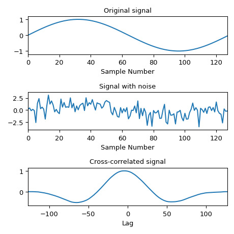
相關用法
- Python SciPy signal.correlate2d用法及代碼示例
- Python SciPy signal.correlation_lags用法及代碼示例
- Python SciPy signal.coherence用法及代碼示例
- Python SciPy signal.convolve2d用法及代碼示例
- Python SciPy signal.convolve用法及代碼示例
- Python SciPy signal.cont2discrete用法及代碼示例
- Python SciPy signal.czt_points用法及代碼示例
- Python SciPy signal.chirp用法及代碼示例
- Python SciPy signal.cheb2ord用法及代碼示例
- Python SciPy signal.cheb1ord用法及代碼示例
- Python SciPy signal.csd用法及代碼示例
- Python SciPy signal.cubic用法及代碼示例
- Python SciPy signal.cheby2用法及代碼示例
- Python SciPy signal.cheby1用法及代碼示例
- Python SciPy signal.cspline1d用法及代碼示例
- Python SciPy signal.check_COLA用法及代碼示例
- Python scipy.signal.czt用法及代碼示例
- Python SciPy signal.choose_conv_method用法及代碼示例
- Python SciPy signal.cwt用法及代碼示例
- Python SciPy signal.cspline1d_eval用法及代碼示例
- Python SciPy signal.cmplx_sort用法及代碼示例
- Python SciPy signal.check_NOLA用法及代碼示例
- Python SciPy signal.residue用法及代碼示例
- Python SciPy signal.iirdesign用法及代碼示例
- Python SciPy signal.max_len_seq用法及代碼示例
注:本文由純淨天空篩選整理自scipy.org大神的英文原創作品 scipy.signal.correlate。非經特殊聲明,原始代碼版權歸原作者所有,本譯文未經允許或授權,請勿轉載或複製。