Python scipy.signal.czt用法及代碼示例

用法: scipy.signal.czt(x, m=None, w=None, a=1 + 0j, *, axis=- 1)

計算 Z 平麵中圍繞螺旋的頻率響應。

參數：

x：數組: 要轉換的信號。
m： int 可選: 所需的輸出點數。默認是輸入數據的長度。
w：複雜的，可選的: 每個步驟中點之間的比率。這必須是精確的，否則累積的誤差會降低輸出序列的尾部。默認為圍繞整個單位圓的等距點。
a：複雜的，可選的: 複平麵的起點。默認為 1+0j。
axis： int 可選: 計算 FFT 的軸。如果未給出，則使用最後一個軸。

out： ndarray: 一個與 x 維度相同的數組，但轉換後的軸的長度設置為 m。

注意：

選擇默認值使得 signal.czt(x) 等效於 fft.fft(x) ，如果 m > len(x) ，則 signal.czt(x, m) 等效於 fft.fft(x, m) 。

如果需要重複轉換，請使用CZT 構造一個專門的轉換函數，無需重新計算常量即可重複使用。

一個示例應用是在係統識別中，反複評估係統的z-transform 的小片段，在預計存在極點的位置周圍，以改進對極點真實位置的估計。 [1]

參考：

scipy.signal.czt：

Steve Alan Shilling，“啁啾 z-transform 及其應用的研究”，第 20 頁(1970 年)https://krex.k-state.edu/dspace/bitstream/handle/2097/7844/LD2668R41972S43.pdf

例子：

生成正弦曲線：

>>> f1, f2, fs = 8, 10, 200  # Hz
>>> t = np.linspace(0, 1, fs, endpoint=False)
>>> x = np.sin(2*np.pi*t*f2)
>>> import matplotlib.pyplot as plt
>>> plt.plot(t, x)
>>> plt.axis([0, 1, -1.1, 1.1])
>>> plt.show()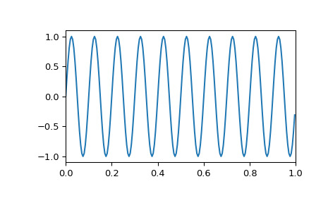

它的離散傅裏葉變換將所有能量都放在一個頻率倉中：

>>> from scipy.fft import rfft, rfftfreq
>>> from scipy.signal import czt, czt_points
>>> plt.plot(rfftfreq(fs, 1/fs), abs(rfft(x)))
>>> plt.margins(0, 0.1)
>>> plt.show()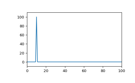

但是，如果正弦曲線是logarithmically-decaying：

>>> x = np.exp(-t*f1) * np.sin(2*np.pi*t*f2)
>>> plt.plot(t, x)
>>> plt.axis([0, 1, -1.1, 1.1])
>>> plt.show()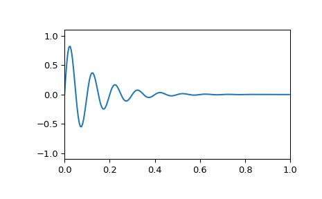

DFT 會有頻譜泄漏：

>>> plt.plot(rfftfreq(fs, 1/fs), abs(rfft(x)))
>>> plt.margins(0, 0.1)
>>> plt.show()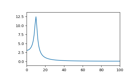

雖然 DFT 總是圍繞單位圓對 z-transform 進行采樣，但啁啾 z-transform 允許我們沿著任何對數螺旋對 Z-transform 進行采樣，例如半徑小於單位的圓：

>>> M = fs // 2  # Just positive frequencies, like rfft
>>> a = np.exp(-f1/fs)  # Starting point of the circle, radius < 1
>>> w = np.exp(-1j*np.pi/M)  # "Step size" of circle
>>> points = czt_points(M + 1, w, a)  # M + 1 to include Nyquist
>>> plt.plot(points.real, points.imag, '.')
>>> plt.gca().add_patch(plt.Circle((0,0), radius=1, fill=False, alpha=.3))
>>> plt.axis('equal'); plt.axis([-1.05, 1.05, -0.05, 1.05])
>>> plt.show()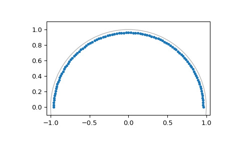

使用正確的半徑，這可以在沒有頻譜泄漏的情況下轉換衰減的正弦曲線(以及其他具有相同衰減率的曲線)：

>>> z_vals = czt(x, M + 1, w, a)  # Include Nyquist for comparison to rfft
>>> freqs = np.angle(points)*fs/(2*np.pi)  # angle = omega, radius = sigma
>>> plt.plot(freqs, abs(z_vals))
>>> plt.margins(0, 0.1)
>>> plt.show()

相關用法

注：本文由純淨天空篩選整理自scipy.org大神的英文原創作品 scipy.signal.czt。非經特殊聲明，原始代碼版權歸原作者所有，本譯文未經允許或授權，請勿轉載或複製。

用法:

參數：

返回：

注意：

參考：

scipy.signal.czt：

例子：