Python numpy random.mtrand.RandomState.normal用法及代码示例

用法： RandomState.normal(loc=0.0, scale=1.0, size=None)

从正态(高斯)分布中抽取随机样本。

正态分布的概率密度函数，首先由De Moivre提出，然后在200年后由Gauss和Laplace分别得出[2]由于其特征形状，通常称为钟形曲线(请参见下面的示例)。

正态分布通常在自然界中发生。例如，它描述了受大量微小随机干扰影响的样本的普遍分布，每种干扰都有其自己独特的分布[2]。

参数：

参数：	loc：： float 或 array_like of floats 分布的平均值(“centre”)。 scale：： float 或 array_like of floats 分布的标准偏差(点差或“width”)。必须为非负数。 size：： int 或 tuple of ints, 可选参数输出形状。如果给定的形状是`(m, n, k)`，然后`m * n * k`抽取样品。如果尺寸是`None`(默认)，如果返回一个值`loc`和`scale`都是标量。除此以外，`np.broadcast(loc, scale).size`抽取样品。
返回值：	out：： ndarray或标量从参数化正态分布中抽取样本。

loc：： float 或 array_like of floats: 分布的平均值(“centre”)。
scale：： float 或 array_like of floats: 分布的标准偏差(点差或“width”)。必须为非负数。
size：： int 或 tuple of ints, 可选参数: 输出形状。如果给定的形状是(m, n, k)，然后m * n * k抽取样品。如果尺寸是None(默认)，如果返回一个值loc和scale都是标量。除此以外，np.broadcast(loc, scale).size抽取样品。

返回值：

out：： ndarray或标量: 从参数化正态分布中抽取样本。

注意：

高斯分布的概率密度为

$p(x) = \frac{1}{\sqrt{ 2 \pi \sigma^2 }} e^{ - \frac{ (x - \mu)^2 } {2 \sigma^2} },$

哪里 $\mu$ 是卑鄙的 $\sigma$ 标准偏差。标准差的平方， $\sigma^2$ ，称为方差。

该函数的平均值处于峰值，并且其“spread”随着标准偏差的增加而增加(该函数在0.65倍时达到最大值) $x + \sigma$ 和 $x - \sigma$ [2])。这意味着numpy.random.normal更有可能返回接近均值的样本，而不是相距较远的样本。

参考文献：

[1]	维基百科，“Normal distribution”，https://en.wikipedia.org/wiki/Normal_distribution

[2]	(1，2，3)P. R. Peebles Jr.，“Central Limit Theorem”，“概率，随机变量和随机信号原理”，第四版，2001年，第51、51、125页。

例子：

从分布中抽取样本：

>>> mu, sigma = 0, 0.1 # mean and standard deviation
>>> s = np.random.normal(mu, sigma, 1000)

验证均值和方差：

>>> abs(mu - np.mean(s))
0.0  # may vary

>>> abs(sigma - np.std(s, ddof=1))
0.1  # may vary

显示样本的直方图以及概率密度函数：

>>> import matplotlib.pyplot as plt
>>> count, bins, ignored = plt.hist(s, 30, density=True)
>>> plt.plot(bins, 1/(sigma * np.sqrt(2 * np.pi)) *
...                np.exp( - (bins - mu)**2 / (2 * sigma**2) ),
...          linewidth=2, color='r')
>>> plt.show()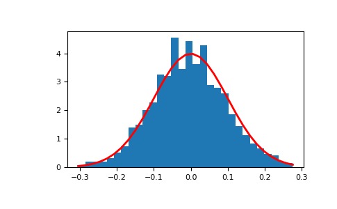

../../../_images/numpy-random-mtrand-RandomState-normal-1_00_00.png

来自N(3，6.25)的Two-by-four个样本数组：

>>> np.random.normal(3, 2.5, size=(2, 4))
array([[-4.49401501,  4.00950034, -1.81814867,  7.29718677],   # random
       [ 0.39924804,  4.68456316,  4.99394529,  4.84057254]])  # random

相关用法

python scipy stats.norm用法及代码示例

注：本文由纯净天空筛选整理自 numpy.random.mtrand.RandomState.normal。非经特殊声明，原始代码版权归原作者所有，本译文未经允许或授权，请勿转载或复制。