Python skimage.transform.hough_line用法及代碼示例

用法: skimage.transform.hough_line(image, theta=None)

執行直線霍夫變換。

參數：

image：(M, N) ndarray: 具有表示邊的非零值的輸入圖像。
theta：1D ndarray of double，可選: 計算變換的角度，以弧度為單位。默認為在 [-pi/2, pi/2) 範圍內均勻分布的 180 個角度的向量。

hspace：uint64 的二維數組: 霍夫變換累加器。
angles：ndarray: 計算變換的角度，以弧度為單位。
distances：ndarray: 距離值。

注意：

原點是原始圖像的左上角。 X 和 Y 軸分別是水平和垂直邊。距離是從原點到檢測線的最小代數距離。可以通過減小 theta 陣列中的步長來提高角度精度。

例子：

生成測試圖像：

>>> img = np.zeros((100, 150), dtype=bool)
>>> img[30, :] = 1
>>> img[:, 65] = 1
>>> img[35:45, 35:50] = 1
>>> for i in range(90):
...     img[i, i] = 1
>>> rng = np.random.default_rng()
>>> img += rng.random(img.shape) > 0.95

應用霍夫變換：

>>> out, angles, d = hough_line(img)

import numpy as np
import matplotlib.pyplot as plt

from skimage.transform import hough_line
from skimage.draw import line

img = np.zeros((100, 150), dtype=bool)
img[30, :] = 1
img[:, 65] = 1
img[35:45, 35:50] = 1
rr, cc = line(60, 130, 80, 10)
img[rr, cc] = 1
rng = np.random.default_rng()
img += rng.random(img.shape) > 0.95

out, angles, d = hough_line(img)

fix, axes = plt.subplots(1, 2, figsize=(7, 4))

axes[0].imshow(img, cmap=plt.cm.gray)
axes[0].set_title('Input image')

angle_step = 0.5 * np.rad2deg(np.diff(angles).mean())
d_step = 0.5 * np.diff(d).mean()
bounds = (np.rad2deg(angles[0]) - angle_step,
          np.rad2deg(angles[-1]) + angle_step,
          d[-1] + d_step, d[0] - d_step)

axes[1].imshow(out, cmap=plt.cm.bone, extent=bounds)
axes[1].set_title('Hough transform')
axes[1].set_xlabel('Angle (degree)')
axes[1].set_ylabel('Distance (pixel)')

plt.tight_layout()
plt.show()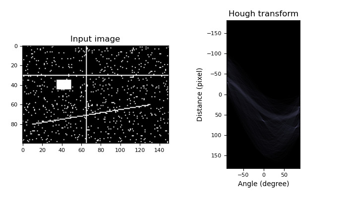

(Source code、png、pdf)

相關用法

注：本文由純淨天空篩選整理自scikit-image.org大神的英文原創作品 skimage.transform.hough_line。非經特殊聲明，原始代碼版權歸原作者所有，本譯文未經允許或授權，請勿轉載或複製。

用法:

參數：

返回：

注意：

例子：